Can numerical differentiation replace backpropagation in a Multilayer Perceptron(MLP)?

Introduction

Is it possible to build a deep learning model without using the backpropagation algorithm?

The answer is yes. In this post, I will build two versions of a Multi-layer Perceptron (MLP) model from scratch: one with backpropagation and the other with numerical differentiation. The model will be trained on the MNIST handwritten digit dataset and will classify each image correctly.

Before we start building the model, there are a few prerequisites:

• First, as this post is about building deep learning models from scratch, I will only use Python, Numpy, and Matplotlib.
• Second, I will not dive deep into the mathematics or algorithms behind the concepts.

What is back propagation?

In machine learning, backpropagation is a gradient estimation method commonly used for training neural networks to compute parameter updates. (from Wiki) It relies on the chain rule. The goal of backpropagation is to update the weights and biases used in the forward pass. When weights and biases are well trained, the model's accuracy increases. To update these parameters, we need to calculate the gradients of each weight and bias because the gradient indicates how much each parameter contributed to the difference between the predicted output and the actual output, also known as the error.

Once we know the error, we have two options:

1. Backpropagation, which propagates weights backward and calculates the gradient of each weight and bias.
2. Numerical differentiation, where we make tiny changes to the parameters and observe how the error changes.

For this implementation, we’ll focus on the second approach, numerical differentiation.

What is numerical differentiation

You may remember the definition of a derivative from high school:

$$f^{\prime }(x)=\underset{h\to 0}{lim}\frac{f(x+h)-f(x)}{h}$$

• h: A very small number
• By taking the limit as h approaches zero, we can find the instantaneous rate of change at a point.

Numerical Differentiation

In the real world, it is challenging to compute derivatives exactly. Instead, we can use numerical differentiation.

Types of Numerical Differentiation:

• Forward Difference:

$$\frac{f(x+h)-f(x)}{h}$$

• Backward Difference:

$$\frac{f(x)-f(x-h)}{h}$$

• Central Difference (more accurate):

$$\frac{f(x+h)-f(x-h)}{2h}$$

We will choose the central difference method because it is more accurate than the others.

How to Apply Numerical Differentiation to Model Training

• $f(x+h)$ : Add very small number h to each parameter x and calculate the error of the model.
• $f(x-h)$ : Subtract very small number h from each parameter x and calculate the error of the model.
• $\frac{f(x+h)-f(x-h)}{2h}$ : Add above 2 numbers and divide into $2h$. It is the gradient of each parameter
• Repeat these steps until all gradients of the parameters are calculated.

Let's Apply Our Idea to Code (feat. MNIST)

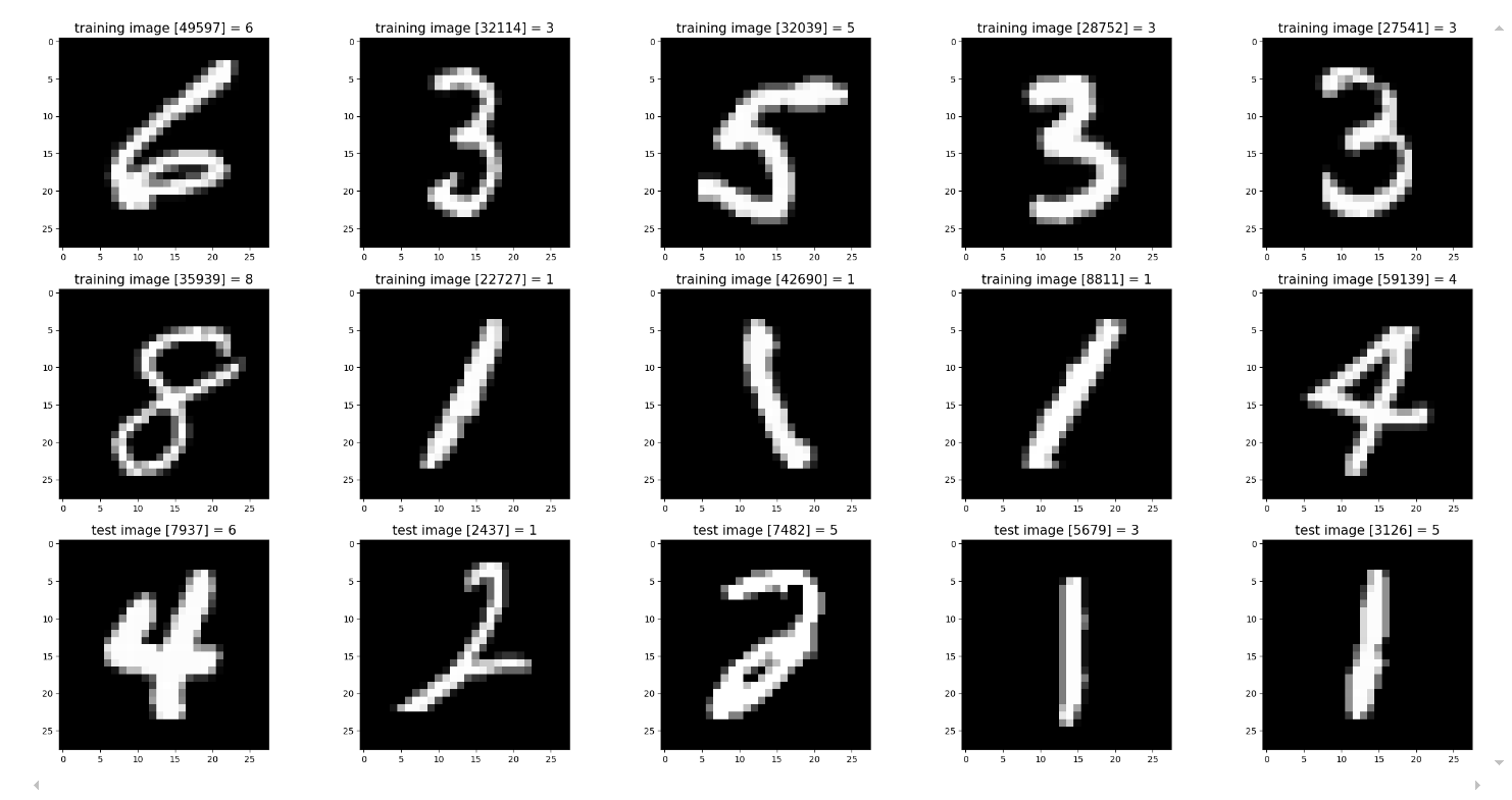
MNIST Dataset

• The MNIST dataset is a collection of handwritten digits, consisting of 60,000 examples for training and 10,000 examples for testing.

Let’s train the model 🤖

• The core concept of numerical differentiation is to compute the gradients (derivatives) of the loss function with respect to the model parameters (such as weights and biases) using numerical methods.
• By adding and subtracting a very small number h (or a small vector or matrix) to each weight and bias, we compute the gradients.
• You can imagine how many times you would have to compute the gradient for a single weight. For example, the shape of W1 (weight) is (784, 50). To calculate the gradient of this weight, we add and subtract h to all elements of W1, which results in 39,200 calculations (784 x 50) for each weight matrix.

Code Snippet

def numerical_gradient(f, y_true, x_data, params, h=1e-4):
    gradients = {}  # Dictionary to store the derivative results for each parameter (W, b)

    for key in params:  # Iterate over each parameter (W1, W2, b1, b2)
        param = params[key]  # Select the current parameter
        grad = np.zeros_like(param)  # Create a gradient array of the same shape as the parameter

        if param.ndim == 1:  # If the parameter is a bias (vector)
            for i in range(param.shape[0]):  # Iterate over each element
                temp_params = params.copy()
                param_plus = param.copy()
                param_minus = param.copy()

                param_plus[i] += h  # Add h to b_i
                param_minus[i] -= h  # Subtract h from b_i

                # Calculate the loss with the bias updated
                temp_params[key] = param_plus
                loss_plus = f(y_true, x_data, temp_params)  
                temp_params[key] = param_minus
                loss_minus = f(y_true, x_data, temp_params)  

                grad[i] = (loss_plus - loss_minus) / (2 * h)  # Compute the central difference

        else:  # If the parameter is a weight (matrix)
            for i in range(param.shape[0]):  # Iterate over rows
                for j in range(param.shape[1]):  # Iterate over columns
                    temp_params = params.copy()
                    param_plus = param.copy()
                    param_minus = param.copy()

                    param_plus[i, j] += h  # Add h to w_ij
                    param_minus[i, j] -= h  # Subtract h from w_ij

                    # Calculate the loss with the weight updated
                    temp_params[key] = param_plus
                    loss_plus = f(y_true, x_data, temp_params)  
                    temp_params[key] = param_minus
                    loss_minus = f(y_true, x_data, temp_params) 

                    grad[i, j] = (loss_plus - loss_minus) / (2 * h)  # Compute the central difference

        gradients[key] = grad  # Store the computed gradient

    return gradients  # Return all gradients

Result

Prerequisites

• Model = Multi-layer perceptron
• Epoch = 50
• Batch size = 100
• Number of Layers = 2 (Input layer, Output layer)
• Parameters = 2 weights, 2 biases
• Loss function = Cross-Entropy Error
• Activation function = Sigmoid

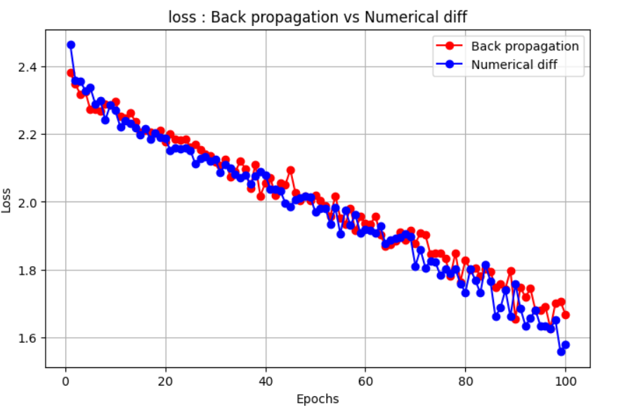
Loss

Test Accuracy

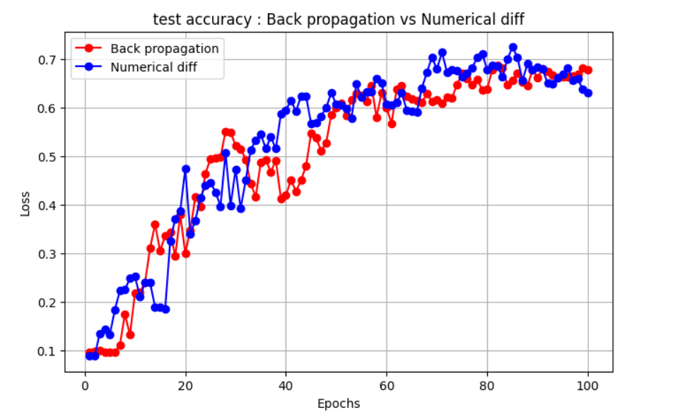
Method	Epochs ⏳	Elapsed Time ⏱️	Loss 📉	Test Accuracy 🎯
Backpropagation	100	3.1s	1.6676	0.6783
Numerical Differentiation	100	141m 55.3s	1.5788	0.6309

Conclusion

You can see how much time it takes to train a 2-layer model when using numerical differentiation to compute the loss gradients. This approach is much slower than backpropagation, but it gives an interesting perspective on how optimization works without the use of advanced optimization techniques.

If you want to check the full code, click here.